3 Results
3.1 Data Tables
| Lesson | Control | MCI | Total |
|---|---|---|---|
|
Pasta |
5 | 6 | 11 |
|
Swahili 1 |
4 | 4 | 8 |
|
Flowers |
5 | 4 | 9 |
|
European Capitals 1 |
4 | 6 | 10 |
|
Birds |
4 | 5 | 9 |
|
Newspapers |
5 | 7 | 12 |
|
Asian Flags |
5 | 7 | 12 |
|
Folktales |
4 | 5 | 9 |
|
Maps |
6 | 7 | 13 |
|
US Towns 1 |
4 | 6 | 10 |
|
Art |
5 | 7 | 12 |
|
Hindu Gods |
6 | 7 | 13 |
|
Cheese |
4 | 5 | 9 |
| Participant | Group | Lessons | AVG | Pasta | Swahili | Flowers | Capitals | Birds | News | Flags | Folktales | Maps | Towns | Art | Hindi | Cheese |
|---|---|---|---|---|---|---|---|---|---|---|---|---|---|---|---|---|
| 69419 | Control | 8 | 15.00 | 15 | 0 | 15 | 0 | 15 | 15 | 0 | 15 | 0 | 15 | 15 | 0 | 15 |
| 69414 | Control | 13 | 14.92 | 15 | 15 | 15 | 15 | 15 | 15 | 15 | 14 | 15 | 15 | 15 | 15 | 15 |
| 69418 | Control | 13 | 14.77 | 15 | 15 | 15 | 15 | 15 | 15 | 15 | 15 | 12 | 15 | 15 | 15 | 15 |
| 69410 | Control | 12 | 14.58 | 15 | 15 | 15 | 15 | 13 | 15 | 15 | 12 | 15 | 15 | 15 | 15 | 0 |
| 69425 | Control | 4 | 13.50 | 0 | 0 | 0 | 0 | 0 | 0 | 0 | 13 | 14 | 0 | 14 | 13 | 0 |
| 69415 | Control | 11 | 6.91 | 7 | 8 | 12 | 7 | 6 | 6 | 5 | 6 | 0 | 5 | 6 | 0 | 8 |
| 69417 | MCI | 13 | 13.92 | 12 | 15 | 15 | 15 | 13 | 15 | 15 | 14 | 15 | 15 | 14 | 9 | 14 |
| 69427 | MCI | 10 | 13.90 | 15 | 15 | 15 | 15 | 14 | 15 | 0 | 15 | 0 | 9 | 15 | 0 | 11 |
| 70930 | MCI | 12 | 12.83 | 9 | 10 | 0 | 12 | 12 | 13 | 15 | 15 | 15 | 15 | 12 | 15 | 11 |
| 70925 | MCI | 1 | 11.00 | 11 | 0 | 0 | 0 | 0 | 0 | 0 | 0 | 0 | 0 | 0 | 0 | 0 |
| 69412 | MCI | 7 | 10.86 | 10 | 0 | 10 | 0 | 11 | 0 | 12 | 8 | 0 | 14 | 0 | 0 | 11 |
| 69411 | MCI | 10 | 9.40 | 7 | 8 | 15 | 14 | 10 | 8 | 0 | 0 | 6 | 0 | 7 | 8 | 11 |
| 69421 | MCI | 8 | 8.12 | 0 | 0 | 0 | 13 | 0 | 8 | 7 | 7 | 8 | 7 | 7 | 8 | 0 |
| 71203 | MCI | 4 | 7.75 | 0 | 0 | 0 | 0 | 0 | 0 | 0 | 0 | 0 | 8 | 5 | 8 | 10 |
| 69422 | MCI | 5 | 7.20 | 0 | 0 | 0 | 0 | 13 | 4 | 7 | 6 | 6 | 0 | 0 | 0 | 0 |
| 69423 | MCI | 6 | 6.33 | 0 | 0 | 0 | 0 | 7 | 5 | 0 | 4 | 7 | 9 | 6 | 0 | 0 |
3.2 Accuracy
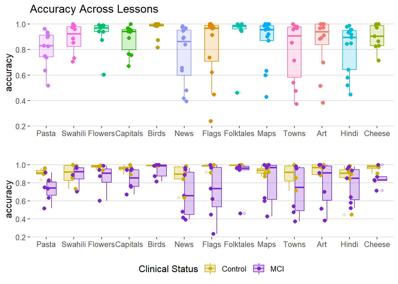
Figure 3.1: Accuracy Across Lessons
Accuracy (fig 3.1) scores were averaged for each participant in each lesson they completed.
Figure 3.2: Accuracy by Participant
This graph is interactive (fig 3.2). Hover over the data points to get a better look at the accuracy scores for each participant. Double click on a participant ID to isolate that participant’s data points.
Figure 3.3: Accuracy by Clinical Status
This graph separates the participants by clinical status (fig 3.3). Participants with MCI tend to have less accuracy compared to the controls.
3.3 Response Time
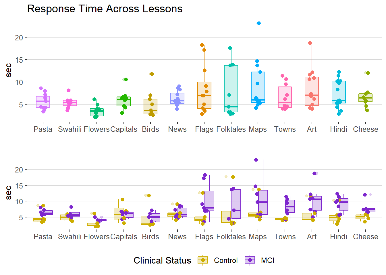
Figure 3.4: Response Time Across Lessons
Response times (fig 3.4) were averaged for each participant in each lesson they completed.
Figure 3.5: Response Time by Participant
Figure 3.5: Response Time by Participant
The graph is interactive (fig 3.5). Hover over the data points to get a better look at the response times for each participant. Double click on a participant ID to isolate that participant’s data points.
Figure 3.6: Response Time by Clinical Status
3.4 Rate of Forgetting
The mean Rate of Forgetting for each participant across all lessons.
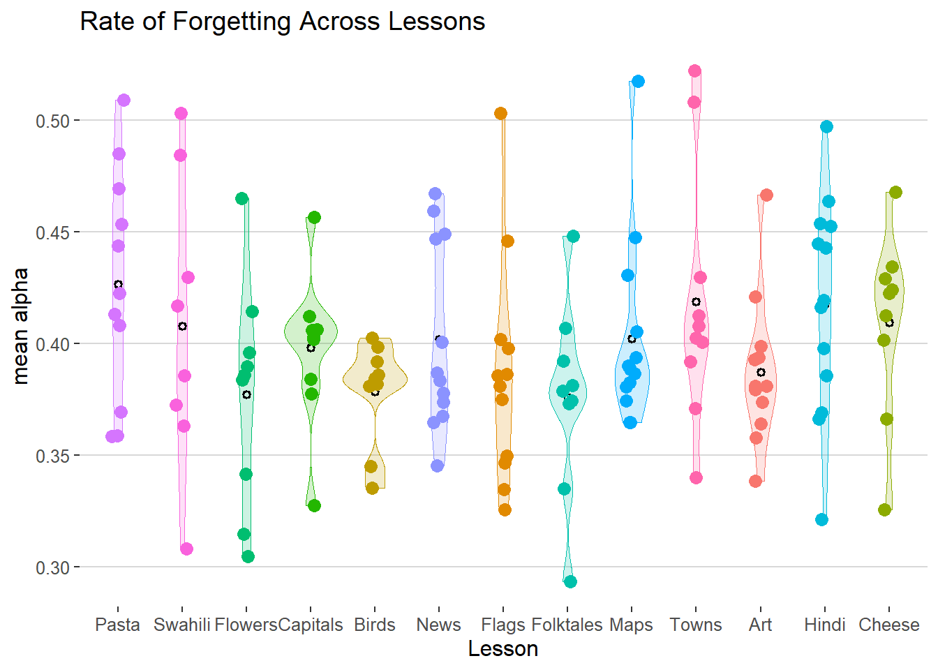
Figure 3.7: Rate of Forgetting Across Lessons
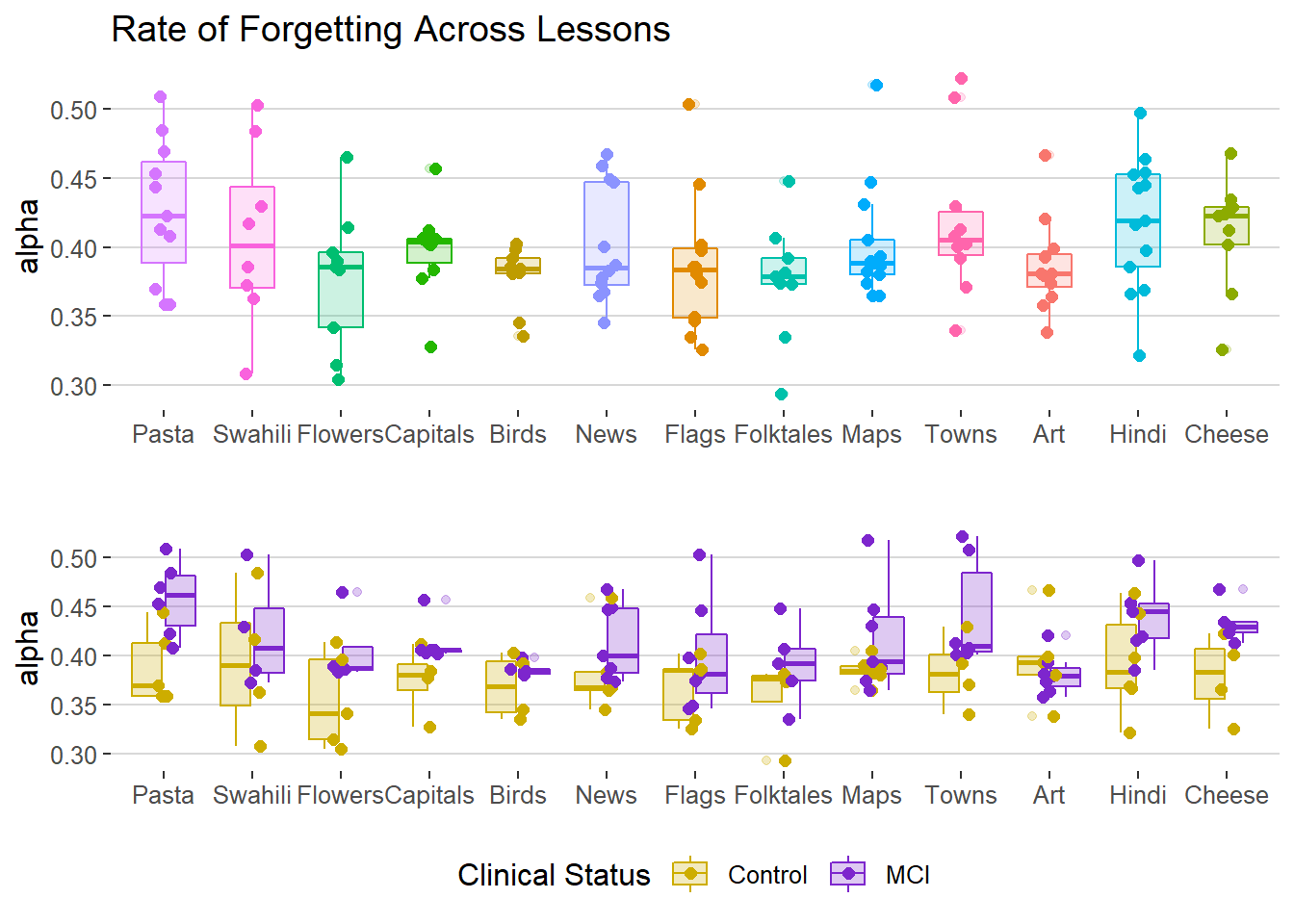
Figure 3.8: Rate of Forgetting Across Lessons
Rates of Forgetting ‘alpha’ (fig 3.8) were averaged for each participant in each lesson they completed.
Figure 3.9: Rate of Forgetting by Participant
Figure 3.10: Rate of Forgetting by Clinical Status
Individuals with MCI tend to have a higher Rate of Forgetting than the age-matched controls (fig 3.10).
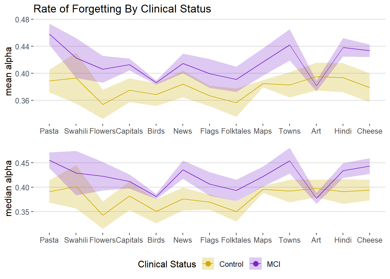
Figure 3.11: Mean and Median Rate of Forgetting by Clinical Status
| stratum | term | df | sumsq | meansq | statistic | p.value |
|---|---|---|---|---|---|---|
| userId | lessonTitle | 12 | 0.1358 | 0.0113 | 0.385 | 0.867 |
| userId | clinicalStatus | 1 | 0.0110 | 0.0110 | 0.374 | 0.650 |
| userId | lessonTitle:clinicalStatus | 1 | 0.0000 | 0.0000 | 0.000 | 0.996 |
| userId | Residuals | 1 | 0.0294 | 0.0294 | NA | NA |
| userId:lessonTitle | lessonTitle | 12 | 0.0341 | 0.0028 | 4.290 | 0.000 |
| userId:lessonTitle | lessonTitle:clinicalStatus | 12 | 0.0152 | 0.0013 | 1.911 | 0.042 |
| userId:lessonTitle | Residuals | 97 | 0.0643 | 0.0007 | NA | NA |
The median Rate of Forgetting for each participant across all lessons.
| stratum | term | df | sumsq | meansq | statistic | p.value |
|---|---|---|---|---|---|---|
| userId | lessonTitle | 12 | 0.1834 | 0.0153 | 0.501 | 0.8169 |
| userId | clinicalStatus | 1 | 0.0102 | 0.0102 | 0.334 | 0.6663 |
| userId | lessonTitle:clinicalStatus | 1 | 0.0001 | 0.0001 | 0.004 | 0.9600 |
| userId | Residuals | 1 | 0.0305 | 0.0305 | NA | NA |
| userId:lessonTitle | lessonTitle | 12 | 0.0502 | 0.0042 | 3.512 | 0.0002 |
| userId:lessonTitle | lessonTitle:clinicalStatus | 12 | 0.0184 | 0.0015 | 1.284 | 0.2405 |
| userId:lessonTitle | Residuals | 97 | 0.1156 | 0.0012 | NA | NA |
3.5 Distribution of Rate of Forgetting
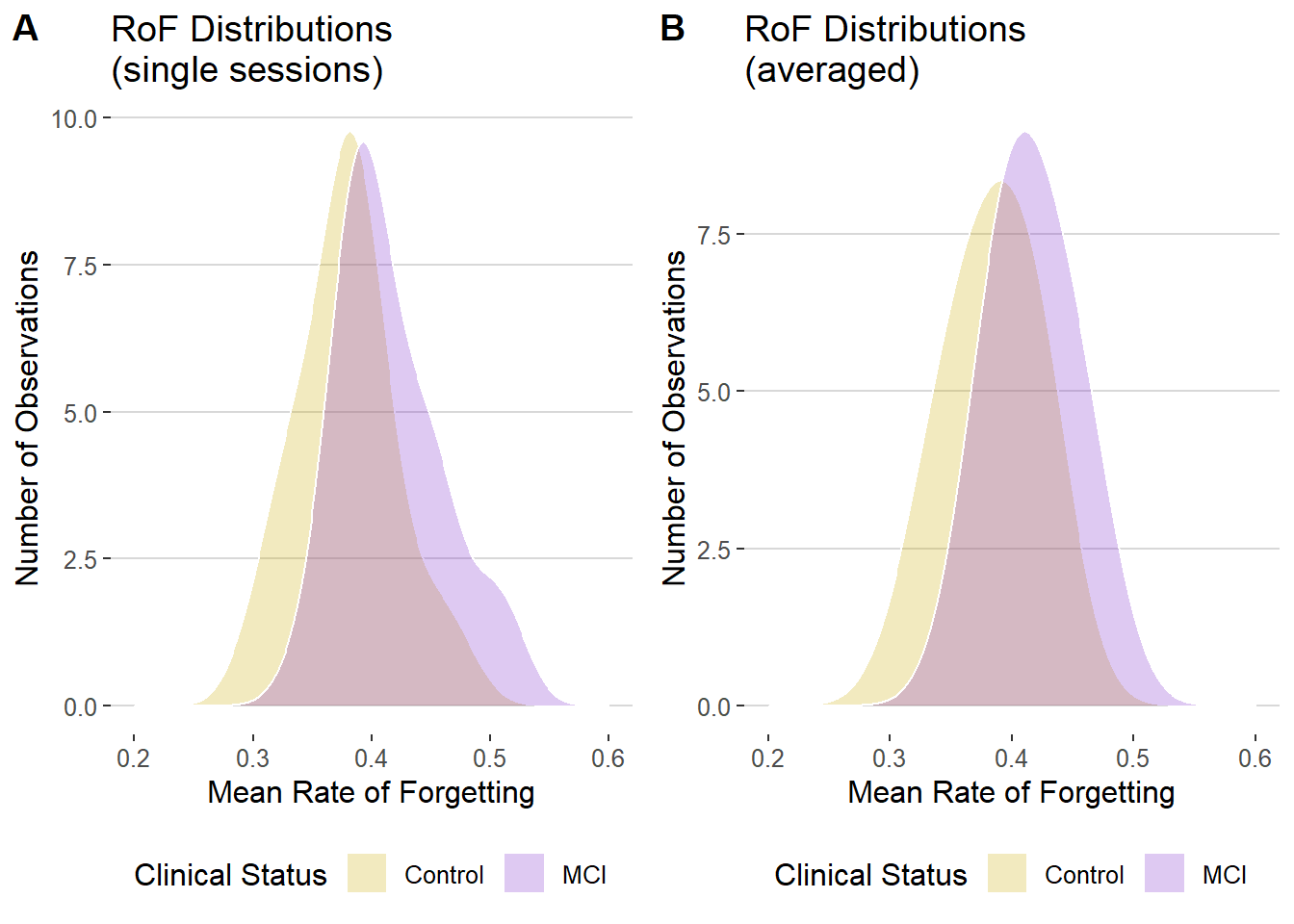
Figure 3.12: Distribution of Rate of Forgetting by Clinical Status
This figure examines the distribution of ROF values for MCIs and controls, either across all sessions (A) or averaged across all sessions (B) (fig 3.12). The biggest point of difference, whether single session or averaged sessions, is at an alpha of about #. The double bump in Figure A is likely due to differences in task difficulty. An interesting point here is that there are some things that are easier for the the MCI than for the controls (shown by that middle section overlap) and this makes it harder for the classifier. If we could build a classifier that has a general idea of difficulty (for instance, have the threshold for “birds”-which is an easier task- be 0.35 instead of 0.37), it would be much better.
3.6 Classification accuracy
One of the most interesting questions which is, “How diagnostic is the Rate of Forgetting?” To analyze a parameter’s classification accuracy, you can plot an ROC curve. This curve will assess the sensitivity and specificity- two components that measure the inherent validity of a diagnostic test- of ROF as a diagnostic tool. First, we examined the ROC curve for just a single 8 minute session of data.
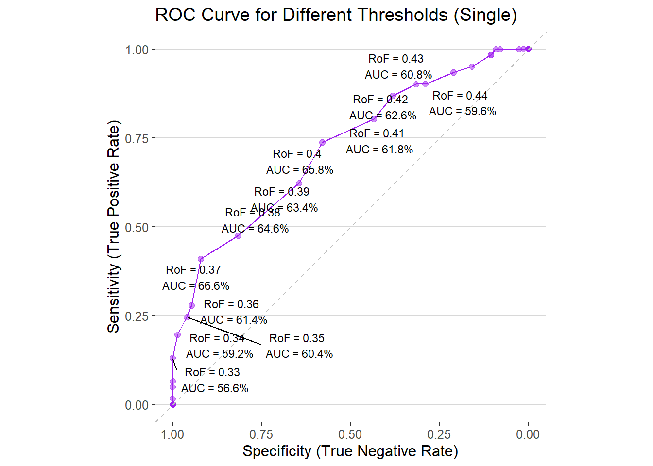
Figure 3.13: Classification Accuracy for different RoF thresholds
This figure visualizes the ROC curve to see the classification accuracy at each RoF threshold (fig 3.13). In this case, having a RoF value of 0.# as the diagnostic threshold- that is people with an RoF of 0.# and up are considered mildly cognitively impaired and people with an RoF less than are healthy controls- gives us a diagnostic classification accuracy of #%. All together though, the global AUC for single session is 0.758.
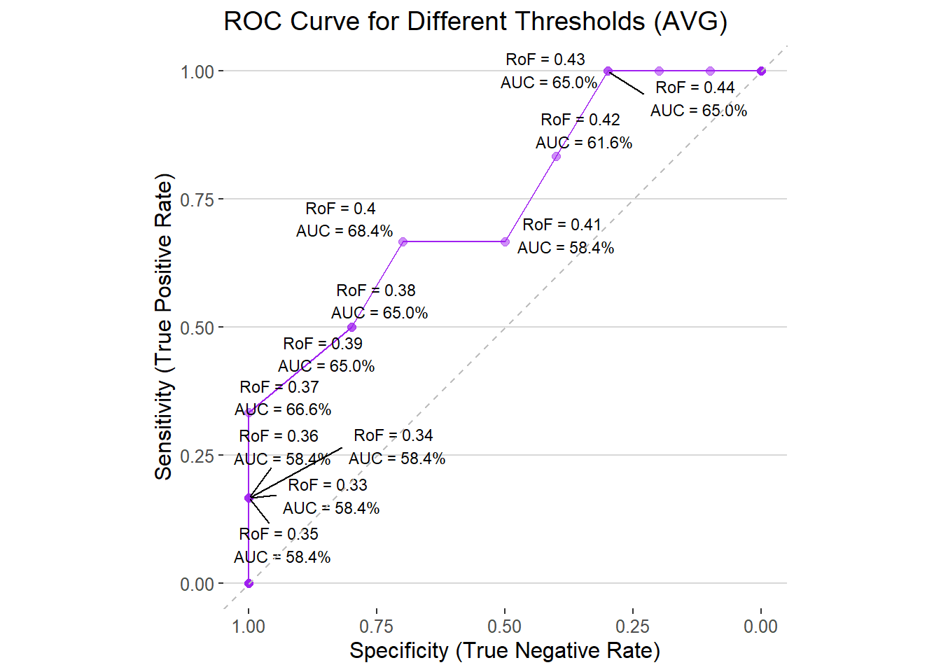
Figure 3.14: Classification Accuracy for different averaged RoF thresholds
This figure visualizes the ROC curve to see the classification accuracy at each RoF threshold (fig 3.14). The global AUC for averaged sessions is 0.784.
3.7 RoF Correlations
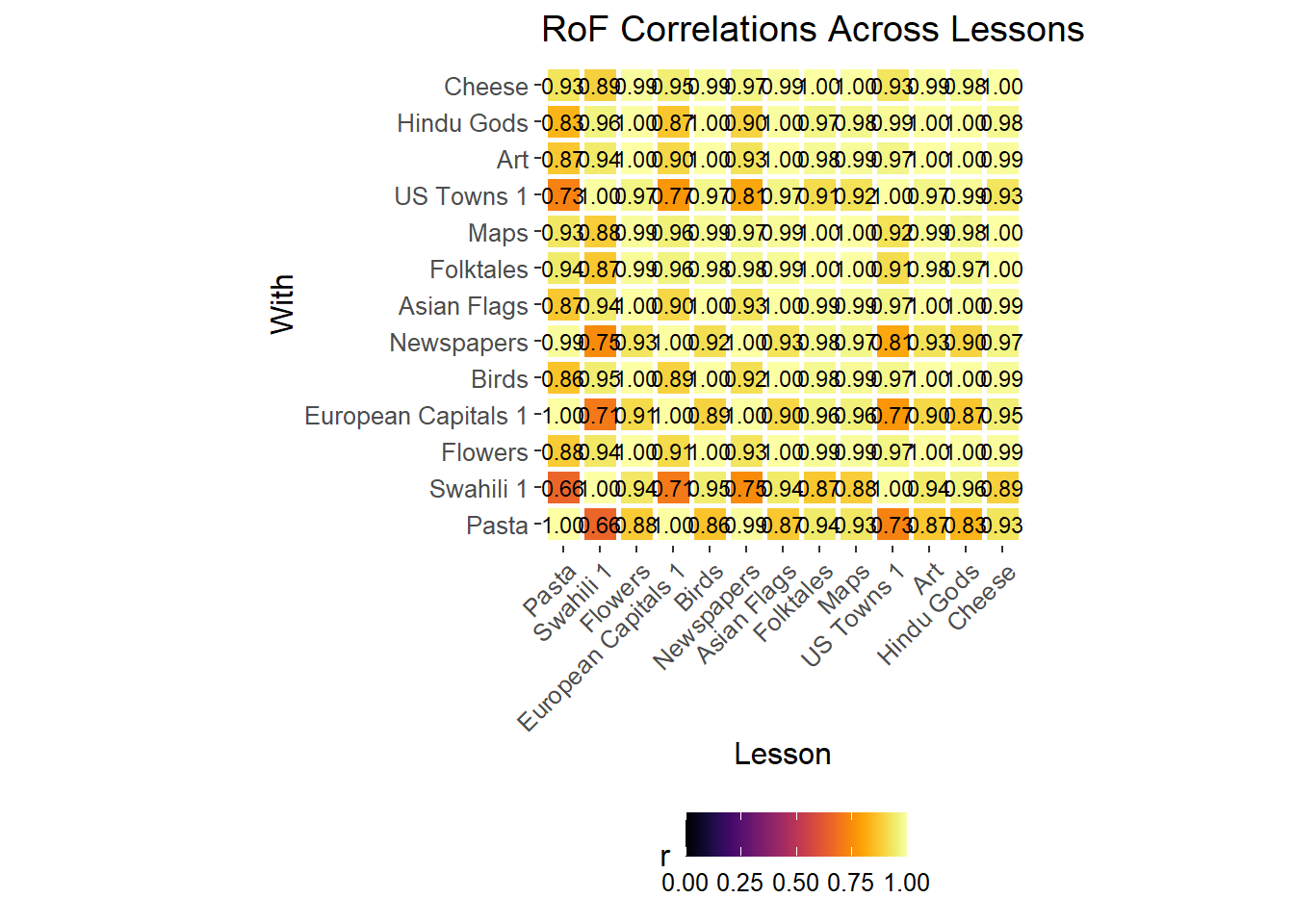
Figure 3.15: RoF Test-Retest Reliability
This figure visualizes the test-retest reliability of the RoF using correlations across materials (fig 3.15). The mean correlation is 0.938.